Hand-outs and Reference Materials

Spinning Phasors

Those that have taken my courses know all about my use of "spinning phasors".

Once you get it, the form \(e^{-j\omega t}\) is so much simpler to use intuitively than its trigonometric equivalent as \(\cos(\omega t) - j\sin(\omega t)\).

(\(e^{-j\omega t}\) represents a phasor with magnitude 1 rotating clockwise on the complex plane with angular frequency \(\omega\) radians/sec).

The details below provide examples as motivation for working with complex signals and "spinning phasors", and concludes with an interactive demo called VectorSpin. To jump to the VectorSpin demo, click here.

SSB Upconverter, Explained with Spinning Phasors

Here is a simple example for those with an RF background: the Single-Sideband (SSB) upconverter, prevalent in both digital and analog systems, that can be made using a quadrature modulator (for example, see the Analog Devices AD8346, and this article by Rick Cushing showing how that part is used for quadrature SSB upconversion).

The SSB upconverter can be used to translate an intermediate frequency (IF) up to one side of a radio-frequency (RF) carrier while attenuating what would appear on the other side of the carrier if we were to simply multiply real sinusoids (see the cosine and sine product rules, which show how multiplying two frequencies produces the sum and the difference). Most explanations for SSB extend those cosine and sine product rules into what ends up being a page of math, with difficulty in reaching intuition as to what is occurring.

The same explanation using "spinning phasors" (we'll use Figure 1 from ADI's application note as a good example):

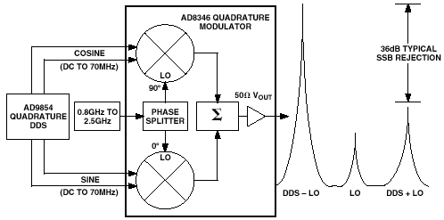
The IF signal is provided in quadrature, so the cosine and sine provided represent a single complex IF waveform as \(e^{-j{\omega_{DDS} t}}\). The Phase Splitter block converts the real RF local oscillator to a single complex RF waveform as \(e^{j\omega_{RF}t}\)

The output is the real portion of the complex product of the two:
\(\mathrm{Re}\{e^{j\omega_{RF} t}\,e^{-j\omega_{DDS} t}\} = \mathrm{Re}\{e^{j(\omega_{RF} - \omega_{DDS}) t}\}\)

Which is \(\cos((\omega_{RF}-\omega_{DDS})t)\) consistent with the larger tone "DDS-LO" in the Analog Devices graphic.

The CTFT, DFT, DTFT Explained With Spinning Phasors (VectorSpin)

The Fourier Transform decomposes time domain waveforms into fundamental "spinning phasor" components. With that representation, a single impulse in one domain (time or frequency) is a spinning phasor in the other domain. To convert from one domain to the other, each impulse is treated as a spinning phasor in the opposite domain and added, via superposition, to all the other phasors. The summation of all these phasors, each spinning at its own rate and starting at its own phase, reconstructs the complete waveform in that domain. Where the phasors reinforce, the waveform has energy; where they cancel, it goes to zero. This is the entire mechanism of the transform.

Example 1: The DFT

The Discrete Fourier Transform shows us the magnitude and starting phase for time domain spinning phasors, each with constant magnitude and spinning at a constant rate, with each an integer multiple (including zero) of the "fundamental frequency". It's really cool how we can come up with any sequence of arbitrary complex samples in the time domain, and the DFT of that sequence is the magnitude and starting phase for that set of spinning phasors, that when we add them all up in the time domain, the resulting vector will pass through each of those complex samples exactly at the given time in the sequence.

Try it! To see this in action in the VectorSpin animation below, select 'Time' for the Input Array and enter any desired sequence of complex numbers using the format 1j to represent the imaginary component, with each number separated by commas (example: 1, 2+3j, 3). Select 'Time Domain' for IQ Mode to be able to view the individual spinning phasors in time corresponding to the DFT result on the right. Notice how the sum of the phasors goes through the entered sequence exactly, at the correct time in the sequence

Example 2: The DTFT and FIR Filters

The frequency response for FIR filters, as a continuous function in the frequency domain providing the magnitude and phase response of the filter versus frequency, is the Discrete Time Fourier Transform (DTFT) for the filter's time domain impulse response, which is the coefficients of the filter itself.

This time domain impulse response is a series of impulses in the time domain. As we learned above, each impulse in one domain is a spinning phasor in the other domain. So a simple 2-tap FIR filter such as \(1 + z^{-1}\) is the sum of two phasors in the frequency domain: One with magnitude 1 that doesn't rotate, and the other with magnitude 1 that rotates once as the frequency goes from DC to the sampling rate.

Try it! To see this in action in the VectorSpin animation below, select 'Time' for the Input Array and enter 1,1 as the time domain sequence, corresponding to the taps of our simple FIR filter. Select 'Freq Domain' for IQ Mode to be able to view the individual spinning phasors in frequency corresponding to the DTFT result on the right. The frequency range shown corresponds to the range from DC to the sampling rate, and thus we see out to Nyquist (half the sampling rate) that the FIR filer given with the transfer function \(H(z)=1+z^{-1}\) is indeed a low pass filter. Change it to be 1, -1 and see how it is now a high pass filter.

Like what you see? These concepts and much more are covered in detail in the Signal Processing for Wireless Communications course, where we build from the ground up complete intuition for signal processing usable in many fields beyond wireless itself. The only prerequisite is the undergraduate engineering Signals and Systems course, and I'll be there to help you through any questions you may have.

To link directly to VectorSpin use: https://vectorspin.dsp-coach.com